外觀
視覺化 › Matplotlib › 散布圖
散布圖 (Scatter Plot)
散布圖呈現兩個連續變數的關係:方向、強度、是否非線性、有無分群與離群值。相關係數只是一個數字,散布圖才看得到形狀(見 雙變數分析)。
python
import matplotlib.pyplot as plt
import numpy as np
import seaborn as sns

iris = sns.load_dataset("iris")
x, y = iris["sepal_length"], iris["petal_length"]

fig, axes = plt.subplots(1, 3, figsize=(14, 4), layout="constrained")

# 1. 依類別分組上色:每組各畫一次並給 label
for species, d in iris.groupby("species"):
    axes[0].scatter(d["sepal_length"], d["petal_length"], label=species, alpha=0.7)
axes[0].legend()

# 2. 用顏色 (c) 與大小 (s) 編碼第三、四個變數
sc = axes[1].scatter(x, y, c=iris["petal_width"], s=iris["sepal_width"] * 15,
                     cmap="viridis", alpha=0.7)
fig.colorbar(sc, ax=axes[1], label="Petal width (cm)")

# 3. 線性趨勢線 + 註解單一點
slope, intercept = np.polyfit(x, y, deg=1)
xs = np.linspace(x.min(), x.max(), 100)
axes[2].scatter(x, y, alpha=0.6)
axes[2].plot(xs, slope * xs + intercept, color="tomato", label=f"y = {slope:.2f}x {intercept:+.2f}")
i = y.idxmax()
axes[2].annotate("max petal length", xy=(x[i], y[i]), xytext=(5, 6.5),
                 arrowprops={"arrowstyle": "->", "color": "gray"})
axes[2].legend()

for ax in axes:
ax.set(xlabel="Sepal length (cm)", ylabel="Petal length (cm)")| 參數 | 用途 |
|---|---|
c= | 顏色;給數值欄位時依 cmap 對應,需加 colorbar |
s= | 點面積(單位 points²),可對應數值欄位 |
alpha= | 透明度,處理點重疊 |
marker=、edgecolor= | 點形狀與邊框 |
np.polyfit(x, y, deg) | 多項式最小平方擬合;要 CI 或殘差用 Seaborn regplot / statsmodels |
趨勢線要畫在排序過的 x 上(如上面的
xs),直接用原始 x 畫plot會來回連線。
點太多:Overplotting
基因表現(數萬個基因)、單細胞(數十萬個細胞)、GWAS(數百萬個 SNP)的散布圖,預設設定會把點疊成一整塊:
python
ax.scatter(x, y, s=2, alpha=0.05, rasterized=True)   # 小點 + 透明;rasterized 讓 PDF 不爆大
ax.hexbin(x, y, gridsize=60, bins="log", cmap="viridis")   # 六角格計數,log 色階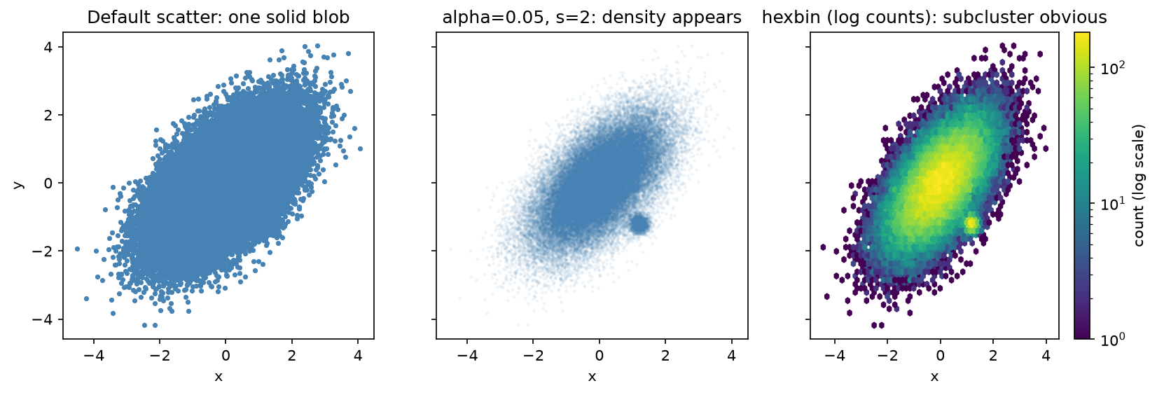
50,000 個點中藏了一個 1,500 點的密集小群。預設畫法只看到一整團;調小點與透明度後密度浮現;hexbin(log 計數)把小群標得最清楚。Seaborn 對應的是 sns.histplot(x=, y=)(2D 直方圖)與 sns.kdeplot(x=, y=)。
相關
| 主題 | 連結 |
|---|---|
| 依類別上色、facet、迴歸線的高階寫法 | Seaborn 關係圖、迴歸圖 |
| 多變數兩兩散布 | Seaborn 矩陣圖 |