外觀
Statistics › 敘述統計 › 雙變數分析
雙變數分析 (Bivariate Analysis)
探討兩個變數之間的關係,方法取決於兩者的型態:
| 變數 A | 變數 B | 描述方法 | 對應檢定 |
|---|---|---|---|
| 數值 | 數值 | 散布圖、Pearson / Spearman / Kendall 相關 | 相關檢定、等級相關 |
| 類別 | 類別 | 交叉表 (cross-tabulation)、分組長條圖 | 卡方檢定 |
| 數值 | 類別 | 分組摘要、分組 boxplot / violin | t 檢定 / ANOVA、Mann-Whitney / Kruskal-Wallis |
| 多個數值 | 多個數值 | 相關矩陣、heatmap、pairplot | 多變量分析 |
相關 ≠ 因果 (correlation ≠ causation)。強相關只代表兩者一起變動,不代表一個造成另一個。
類別 × 類別:交叉表
交叉表 (contingency table) 呈現兩個類別變數的聯合次數。重點是選對標準化方向:
normalize= | 意義 | 回答的問題 |
|---|---|---|
False(預設) | 原始次數 | 各格有幾筆? |
"index" | 每列加總為 1 | 在某性別中,存活比例多少? |
"columns" | 每欄加總為 1 | 在存活者中,男女各佔多少? |
"all" | 全表加總為 1 | 各組合佔全體多少? |
python
import pandas as pd

data = pd.DataFrame({
    "Gender":   ["Male", "Female", "Male", "Female", "Male", "Female"],
    "Survived": ["No",   "Yes",    "Yes",  "Yes",    "No",   "No"],
})

pd.crosstab(data["Gender"], data["Survived"], margins=True)          # 次數 + 總計
pd.crosstab(data["Gender"], data["Survived"], normalize="index")     # 列比例
# Survived     No    Yes
# Female    0.333  0.667
# Male      0.667  0.333
數值 × 數值:相關係數 (Correlation)
| 方法 | 衡量 | 資料 | 離群值 | 適用 |
|---|---|---|---|---|
| Pearson r | 線性關係 | 連續、近似常態 | 敏感 | 乾淨的數值資料 |
| Spearman ρ | 單調 (monotonic) 關係(用排名算 Pearson) | Ordinal、偏態 | 穩健 | 非常態、有離群值 |
| Kendall τ | 單調關係(一致 / 不一致配對) | Ordinal、小樣本 | 穩健 | 小樣本、很多同分 (ties) |
強度參考(只是經驗值,依領域而定)
| |r| | 強度 |
|---|---|
| < 0.3 | 弱 |
| 0.3 – 0.5 | 中 |
| ≥ 0.5 | 強 |
python
from scipy import stats
from sklearn.datasets import load_iris

df = load_iris(as_frame=True).frame
a, b = df["sepal length (cm)"], df["petal length (cm)"]

r, p = stats.pearsonr(a, b)        # Pearson r 與 p 值
rho, p = stats.spearmanr(a, b)     # Spearman ρ
tau, p = stats.kendalltau(a, b)    # Kendall τ
a.corr(b)                          # pandas 快速版(只有係數)
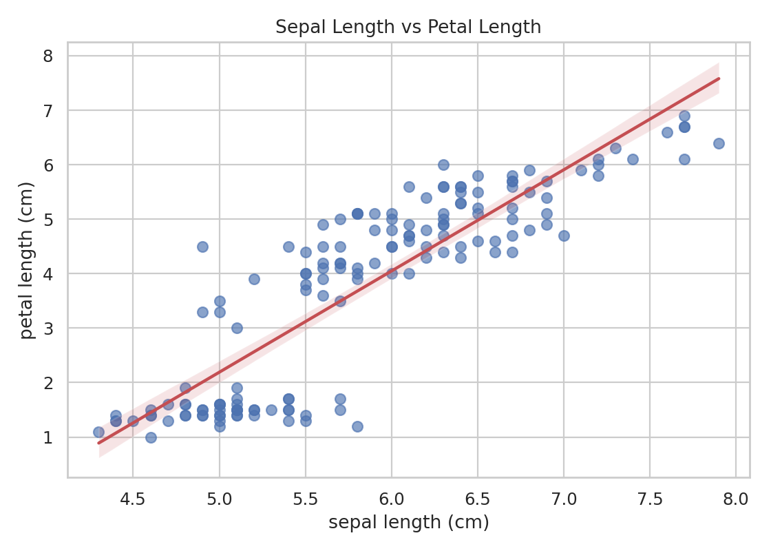
Pearson 的前提:兩者皆為連續變數、關係為線性(看散布圖)、大致常態、無嚴重離群值。不符合時改用 Spearman。
重點
先畫圖:散布圖
Anscombe's Quartet:四組資料相關係數幾乎相同,圖形卻完全不同。先畫圖,再算數字。
python
import matplotlib.pyplot as plt
import seaborn as sns

sns.regplot(x=a, y=b, scatter_kws={"alpha": 0.6}, line_kws={"color": "#c44e52"})
plt.title(f"Sepal vs Petal Length (r = {r:.3f})")
plt.show()| 散布圖 + 迴歸線 | Anscombe's Quartet |
|---|---|
 | 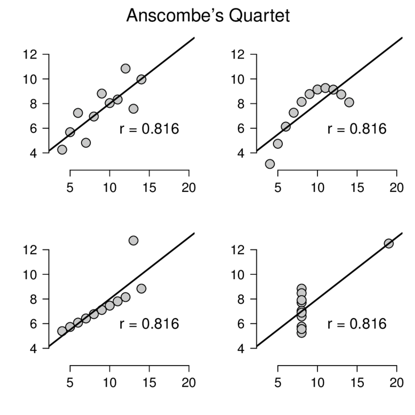 |
Anscombe 圖片來源:ResearchGate
數值 × 類別:分組比較
python
iris = load_iris(as_frame=True)
df = iris.frame
df["species"] = iris.target_names[iris.target]
col = "sepal length (cm)"

# 分組摘要
df.groupby("species")[col].agg(
    n="count", mean="mean", median="median", sd="std",
    iqr=lambda s: s.quantile(0.75) - s.quantile(0.25),
).round(3)
#             n   mean  median     sd    iqr
# setosa     50  5.006     5.0  0.352  0.400
# versicolor 50  5.936     5.9  0.516  0.700
# virginica  50  6.588     6.5  0.636  0.675

# 三種圖
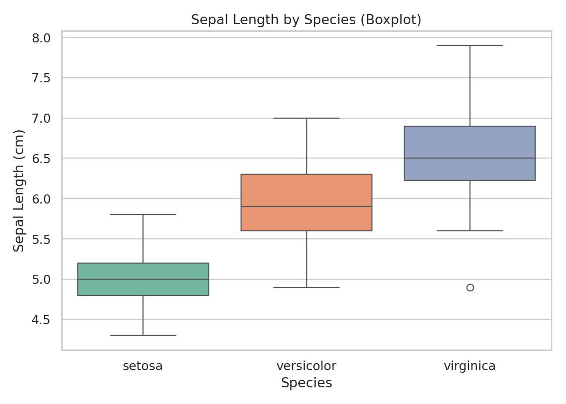
sns.boxplot(x="species", y=col, data=df)                  # 中位數、IQR、離群值
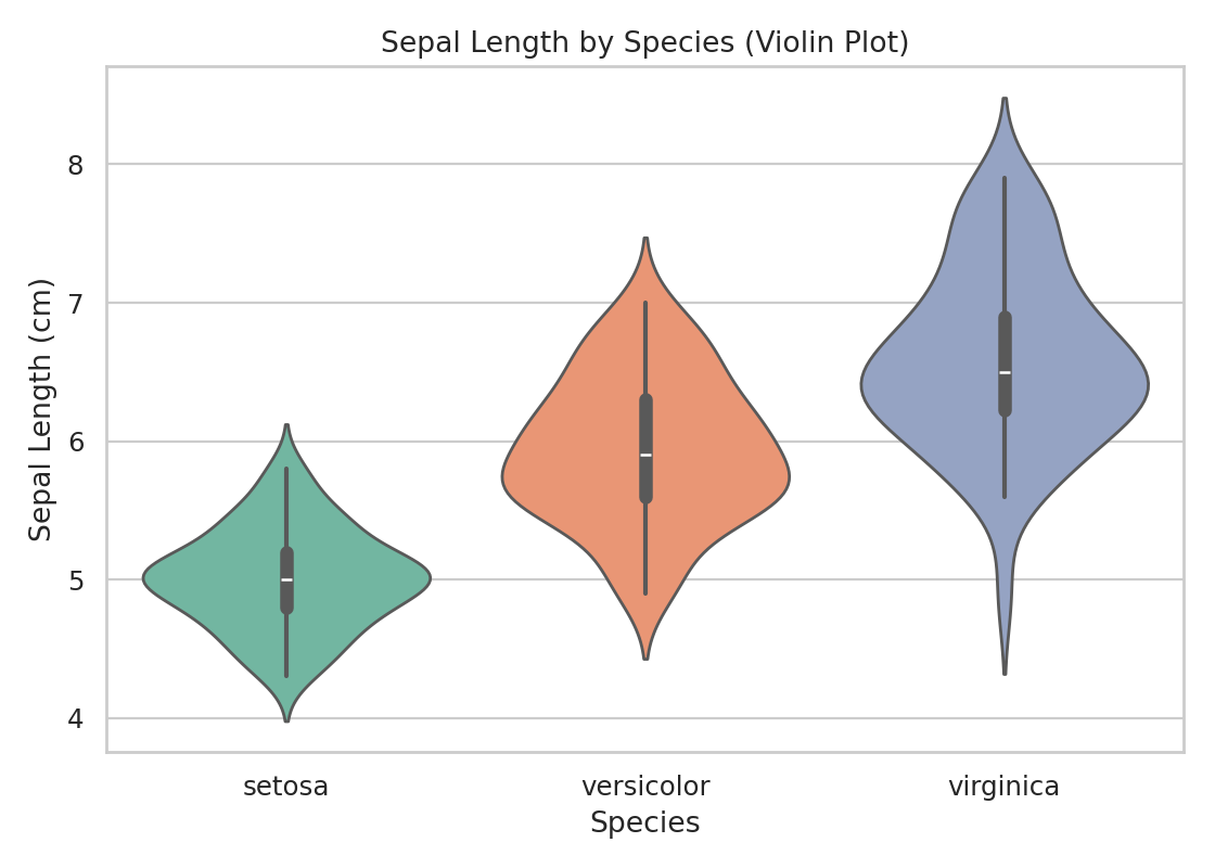
sns.violinplot(x="species", y=col, data=df)               # 分布形狀
sns.barplot(x="species", y=col, data=df, errorbar="sd") # 平均數 ± SD| 圖 | 適合 |
|---|---|
| 分組 boxplot | 比較中位數與分散、找離群值 |
| violin plot | 看各組分布形狀(例如雙峰) |
| 長條圖 + error bar | 比較平均數;務必註明 error bar 是 SD / SE / CI |
| Boxplot | Violin | Bar + error bar |
|---|---|---|
 |  | 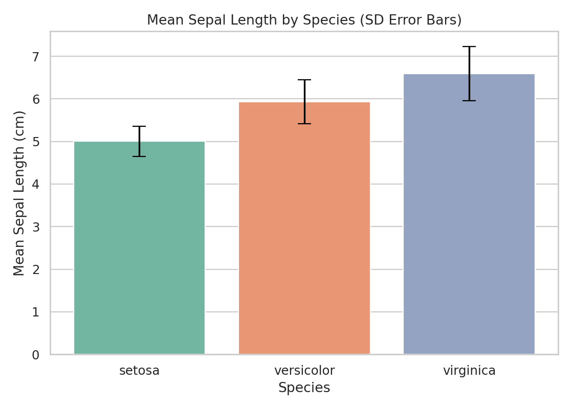 |
樣本少時(例如每組 n = 3 的生物重複),長條圖會隱藏資料點,建議疊加原始點(
sns.stripplot)。
多個數值變數:相關矩陣
python
num_cols = df.select_dtypes("number").columns
corr = df[num_cols].corr(method="pearson")   # 或 "spearman"

# Heatmap
sns.heatmap(corr, annot=True, fmt=".2f", cmap="coolwarm", vmin=-1, vmax=1, center=0, square=True)
plt.show()

# Pairplot:所有變數兩兩散布圖,對角線為分布
sns.pairplot(df, hue="species", diag_kind="kde")
plt.show()| Heatmap | Pairplot |
|---|---|
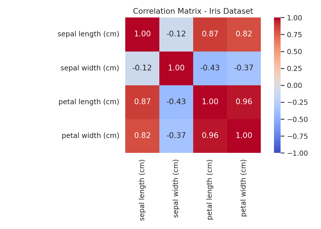 | 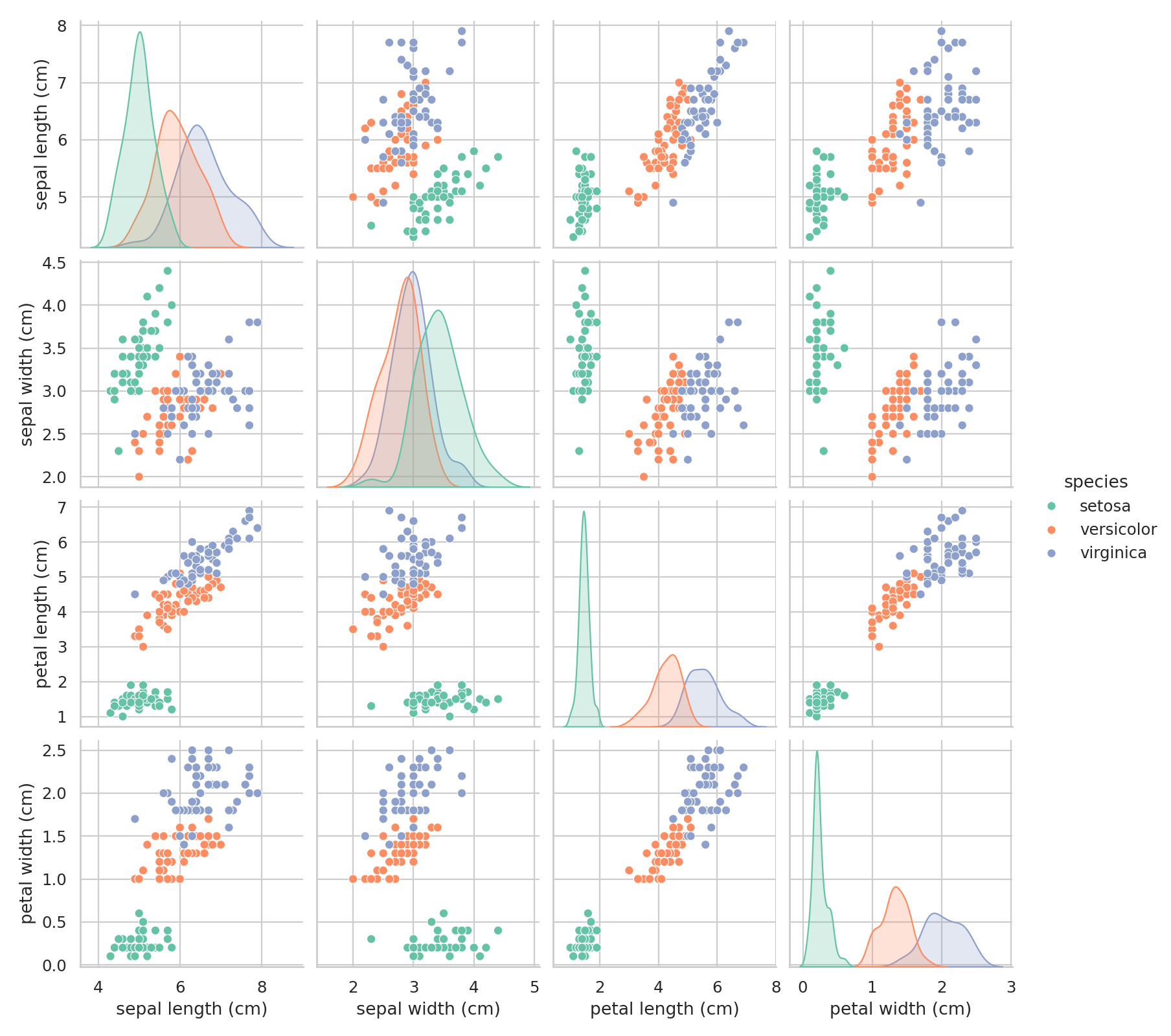 |
解讀關係前的三個問題
- 真的是線性關係嗎?
- 這個關聯是不是被離群值或子群體 (subgroup) 驅動?→ 見 Simpson's paradox,干擾與偏誤
- 是否有第三個變數(干擾因子 confounder)能解釋?
雙變數分析是篩選階段,不是下因果結論的階段。