外觀
Statistics › 時間序列 › 分解
時間序列分解 (Decomposition)
把序列拆成趨勢、季節、殘差,看出模型還需要處理哪些結構,也更容易發現異常或結構改變。分解是描述性的,不保證能產生好的預測。
加法 vs 乘法
| 模型 | 公式 | 何時用 |
|---|---|---|
| 加法 (additive) | Yₜ = Tₜ + Sₜ + Rₜ | 季節振幅固定 |
| 乘法 (multiplicative) | Yₜ = Tₜ × Sₜ × Rₜ | 季節振幅隨水準等比例變大(喇叭形) |
取 log 可把乘法轉成加法:log Y = log T + log S + log R,所以常先 log 再做加法分解。
Classical vs STL
| Classical(移動平均) | STL(Seasonal-Trend decomposition using LOESS) | |
|---|---|---|
| 端點的趨勢 | 缺失(前後 m/2 期為 NaN) | 有 |
| 季節型態 | 固定不變 | 可隨時間演變 |
| 對離群值 | 敏感 | robust=True 可降低影響 |
| 多重季節性 | 不行 | 不行(用 MSTL) |
| 乘法 | 直接支援 | 先取 log |
| 建議 | 快速探索、教學 | 實務預設 |
python
import numpy as np
import statsmodels.api as sm
from statsmodels.tsa.seasonal import seasonal_decompose, STL

series = sm.datasets.co2.load_pandas().data["co2"].resample("MS").mean().interpolate()

classical = seasonal_decompose(series, model="additive", period=12)
classical.plot()

res = STL(series, period=12, robust=True).fit()
res.plot()                                  # observed / trend / seasonal / resid

# 去季節化序列(官方「季節調整後失業率」就是這個)
seasonally_adjusted = series - res.seasonal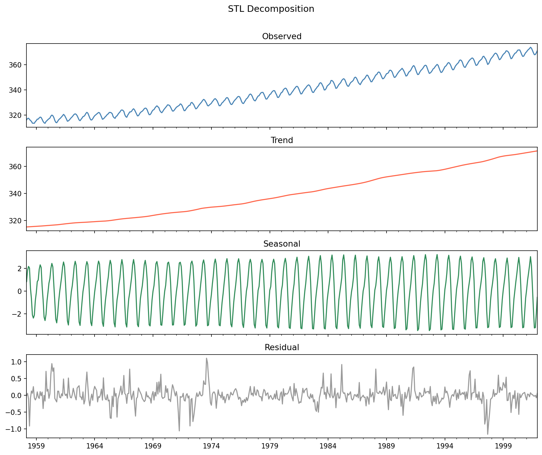
| STL 參數 | 說明 |
|---|---|
period | 季節週期(月資料 12、日資料 7),必填 |
robust | 有離群值時設 True |
seasonal | 季節成分平滑度(奇數,越大越平滑) |
trend | 趨勢平滑度(奇數,需 > period) |
成分強度 (Wang, Smith & Hyndman, 2006)
範圍 0–1;> 0.6 表示該成分顯著,需要在模型中處理。
python
var_r = np.var(res.resid)
strength_trend = max(0, 1 - var_r / np.var(res.trend + res.resid))
strength_seasonal = max(0, 1 - var_r / np.var(res.seasonal + res.resid))
比較多條序列的趨勢
多條序列各自分解後,把同一成分(如趨勢)組成 DataFrame,再看哪些序列「一起動」:
python
import pandas as pd
import seaborn as sns
from statsmodels.tsa.seasonal import STL

trend_df = pd.DataFrame({col: STL(jobs[col], period=12).fit().trend for col in jobs.columns})
trend_corr = trend_df.corr(method="spearman")
sns.clustermap(trend_corr, annot=True, linewidth=0.4)
比原始序列直接算相關更好:去掉季節成分後,相關不會被共同的季節循環灌水。
分解之後
| 觀察 | 下一步 |
|---|---|
| 強趨勢、弱季節 | 差分或趨勢模型 |
| 強季節 | 季節差分、SARIMA、STL + ARIMA |
| 殘差有大尖峰 | 調查異常或介入事件 |
| 殘差仍有自相關 | 進入 ARIMA 建模 |