外觀
Statistics › 推論統計 › 信賴區間
信賴區間 (Confidence Intervals, CI)
信賴區間給出母體參數的合理範圍,同時表達點估計與不確定性。比起只報 p 值,CI 還告訴你效果的大小、方向與精確度。
「95% 信賴」是什麼意思?
| 說法 | |
|---|---|
| ✅ 正確 | 若重複抽樣並每次建構區間,長期下約 95% 的區間會包含真實參數 |
| ❌ 錯誤 | 「μ 有 95% 機率落在這個區間」:μ 是固定值,這個區間要嘛包含、要嘛不包含 |
| ❌ 錯誤 | 「95% 的資料落在這個區間」:那是預測區間 / 參考範圍,不是 CI |
| ❌ 錯誤 | 「兩組 CI 有重疊 → 沒有顯著差異」:差異的顯著性要看差值的 CI |
機率描述的是建構區間的程序,不是某一個特定區間。
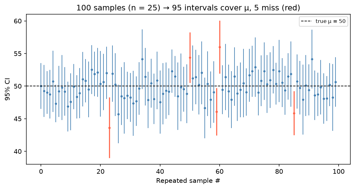 比喻:撒網 100 次,約 95 次網住魚;但任何一次網要嘛有魚、要嘛沒有。
想要「參數有 95% 機率落在區間內」這種解讀,要用貝氏的 可信區間 (credible interval)。
平均數的 CI
| 情況 | 公式 | 臨界值 |
|---|---|---|
| σ 已知(少見) | z | |
| σ 未知(標準情況) | t,df = n − 1 |
| 信賴水準 | α | |
|---|---|---|
| 90% | 0.10 | 1.645 |
| 95% | 0.05 | 1.960 |
| 99% | 0.01 | 2.576 |
z vs t:結構相同,差別只在分母用 σ(已知)或 s(估計)。σ 幾乎永遠未知,預設用 t;n 大時 t 自動趨近 z。
python
import numpy as np
import scipy.stats as stats
from sklearn.datasets import load_iris

x = load_iris(as_frame=True).frame["sepal length (cm)"]
n, x_bar, se = len(x), x.mean(), x.std(ddof=1) / np.sqrt(len(x))

# 手算
t_crit = stats.t.ppf(0.975, df=n - 1)
(x_bar - t_crit * se, x_bar + t_crit * se)

# 一行版
stats.t.interval(0.95, df=n - 1, loc=x_bar, scale=se)

# 臨界值速查
stats.norm.ppf(0.975)          # 雙尾 z = 1.96
stats.norm.ppf(0.95)           # 單尾 z = 1.645(用於單尾檢定)
比例的 CI
Wald 公式:
| 方法 | 何時用 |
|---|---|
| Wald(常態近似) | n 大、p̂ 不接近 0 或 1 |
| Wilson | 建議預設,各種 n 與 p̂ 都表現好 |
| Clopper-Pearson(exact) | n 很小;較保守 |
python
from statsmodels.stats.proportion import proportion_confint

proportion_confint(count=82, nobs=150, alpha=0.05, method="wilson")
影響區間寬度的因素
| 因素 | 變化 | CI 寬度 | 直覺 |
|---|---|---|---|
| 樣本數 n | ↑ | ↓ 變窄(∝ 1/√n) | 資料越多越精確 |
| 信賴水準 | ↑(95 → 99%) | ↑ 變寬 | 要更有把握就得撒更大的網 |
| 資料變異 s | ↑ | ↑ 變寬 | 越分散越難定位平均 |
CI 與 p 值的關係
| p 值 | 信賴區間 | |
|---|---|---|
| 回答 | 效果是否統計顯著? | 效果的合理範圍是多少? |
| 資訊 | 二元:顯著 / 不顯著 | 大小 + 方向 + 精確度 |
| 關係 | p < 0.05 ⇔ 95% CI 不包含 H₀ 的值 | 數學上等價 |
CI 為 [0.001, 0.003] 的結果可能「顯著」但毫無實務意義。兩者都報。
視覺化:分組平均數 ± 95% CI
python
import matplotlib.pyplot as plt
import seaborn as sns

iris = load_iris(as_frame=True)
df = iris.frame.assign(species=iris.target_names[iris.target])

sns.pointplot(data=df, x="species", y="sepal length (cm)", errorbar=("ci", 95),
              linestyle="none", capsize=0.2)
plt.title("Mean Sepal Length with 95% CI")
plt.show()要判斷兩組是否不同,請直接算差值的 CI(例如 兩樣本 t 檢定 的輸出),不要用目測重疊判斷。